Outliers are values that significantly differ from other observations in a dataset, potentially suggesting variations in measurement, experimental errors, or the presence of something unique. Simply put, an outlier is an observation that deviates from the general pattern within a sample.
We have two main outliers type:
Univariate: detecting univariate outliers involves examining the distribution of values within a single feature space.
Multivariate: identifying multivariate outliers occurs within an n-dimensional space corresponding to n features. Analyzing distributions in such multidimensional spaces can be challenging for the human brain, necessitating the use of a trained model to perform this task on our behalf.
Methods for replacing and removing outliers
1- Capping: In this approach, we set a threshold for our outlier data, establishing a limit where values above or below a specific threshold are considered outliers. The count of outliers in the dataset corresponds to the number determined by this capping procedure.
2- Trimming: This method involves excluding outlier values from our analysis. Implementing this technique results in a more focused dataset, particularly in situations where there is a notable presence of outliers. Its primary advantage lies in its efficiency, as it is a quick process.
3- Treatment as missing values: By considering outliers as if they were missing observations, treat them in a manner consistent with the treatment of missing values.

Lets do some analysis
Importing necessary libraries:
 #Step-1: Importing Necessary Dependencies

import numpy as np
import pandas as pd
import matplotlib.pyplot as plt
from sklearn.cluster import DBSCAN
import pandas as pd
from collections import Counter
from sklearn.preprocessing import StandardScaler
import numpy as np
import seaborn as sns
Loading data:
df = pd.read_csv('Placement_data_full_class.csv')Do some visualization
plt.figure(figsize=(16,5))
plt.subplot(2,3,1)
sns.distplot(df['degree_p'])
plt.subplot(2,3,2)
sns.distplot(df['salary'])
plt.subplot(2,3,3)
sns.distplot(df['hsc_p'])
plt.subplot(2,3,4)
sns.distplot(df['ssc_p'])
plt.subplot(2,3,5)
sns.distplot(df['mba_p'])
plt.subplot(2,3,6)
sns.distplot(df['etest_p'])
plt.show()
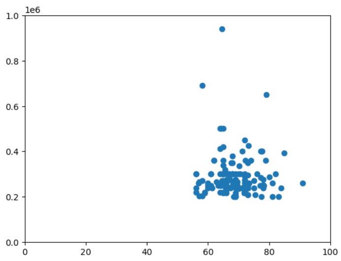
import matplotlib.pyplot as plt
plt.scatter(df['degree_p'],df['salary'])
plt.xlim(0,100)
plt.ylim(0,1000000)
plt.show()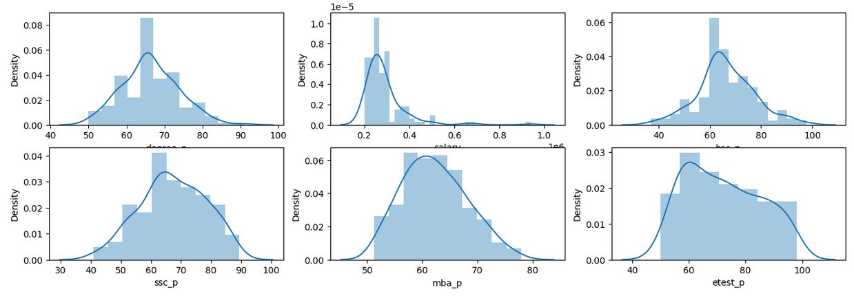
Finding outliers and plot them:
#Step-4: Finding the Boundary Values
Highest_allowed_degree=df['degree_p'].mean() + 3*df['degree_p'].std()
Lowest_allowed_degree=df['degree_p'].mean() - 3*df['degree_p'].std()
Highest_allowed_Salary=df['salary'].mean() + 3*df['salary'].std()
Lowest_allowed_Salary=df['salary'].mean() - 3*df['salary'].std()
print("Highest allowed_degree",Highest_allowed_degree)
print("Lowest allowed_degree : ",Lowest_allowed_degree)
print("Highest allowed Salary",Highest_allowed_Salary)
print("Lowest allowed Salary",Lowest_allowed_Salary)
#Step-5: Finding the Outliers
Outlier_data=df[(df['salary'] > Highest_allowed_Salary) | (df['salary'] < Lowest_allowed_Salary)].append(df[(df['degree_p'] > Highest_allowed_degree) | (df['degree_p'] < Lowest_allowed_degree)])
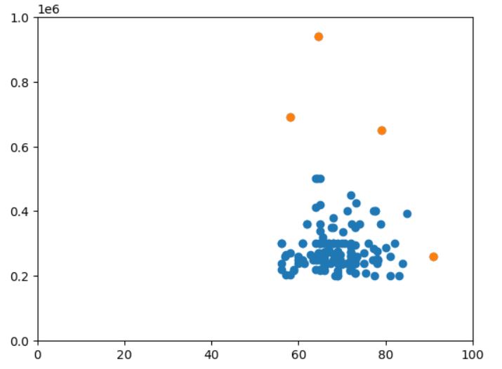
#plot outliers
import matplotlib.pyplot as plt
plt.scatter(df['degree_p'],df['salary'])
plt.scatter(Outlier_data['degree_p'],Outlier_data['salary'])
#changel lim according to your data
plt.xlim(0,100)
plt.ylim(0,1000000)
plt.show()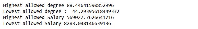
1- Capping
Finding outliers and plotting them:
## Capping

df_c=df.copy()
df_c['degree_p'][df_c['degree_p']>Highest_allowed_degree]=Highest_allowed_degree
df_c['degree_p'][df_c['degree_p']<Lowest_allowed_degree]=Lowest_allowed_degree

df_c['salary'][df_c['salary']>Highest_allowed_Salary]=Highest_allowed_Salary
df_c['salary'][df_c['salary']<Lowest_allowed_Salary]=Lowest_allowed_Salary


#plot outliers
plt.scatter(df_c['degree_p'],df_c['salary'])
plt.xlim(0,100)
plt.ylim(0,1000000)
plt.show()
plt.scatter(df['degree_p'],df['salary'])
plt.scatter(Outlier_data['degree_p'],Outlier_data['salary'])
#changel lim according to your data
plt.xlim(0,100)
plt.ylim(0,1000000)
plt.show()

2- Trimming
## Triming
#just apply pands dataframe filter
df_t=df.copy()
df_t=df_t[(df_t['salary'] < Highest_allowed_Salary) & (df_t['salary'] > Lowest_allowed_Salary)]
df_t=df_t[(df_t['degree_p'] < Highest_allowed_degree) & (df_t['degree_p'] > Lowest_allowed_degree)]
plt.scatter(df_t['degree_p'],df_t['salary'])
plt.xlim(0,100)
plt.ylim(0,1000000)
plt.show()
plt.scatter(df['degree_p'],df['salary'])
plt.scatter(Outlier_data['degree_p'],Outlier_data['salary'])
#changel lim according to your data
plt.xlim(0,100)
plt.ylim(0,1000000)
plt.show()
Considering outliers as missing values:
## Considering as missing value
df_n=df.copy()
df_n['salary'][(df_n['salary'] >= Highest_allowed_Salary) | (df_n['salary'] <= Lowest_allowed_Salary)]=np.nan
df_n['degree_p'][(df_n['degree_p'] >= Highest_allowed_degree) | (df_n['degree_p'] <= Lowest_allowed_degree)]=np.nan
Ways for handling outliers
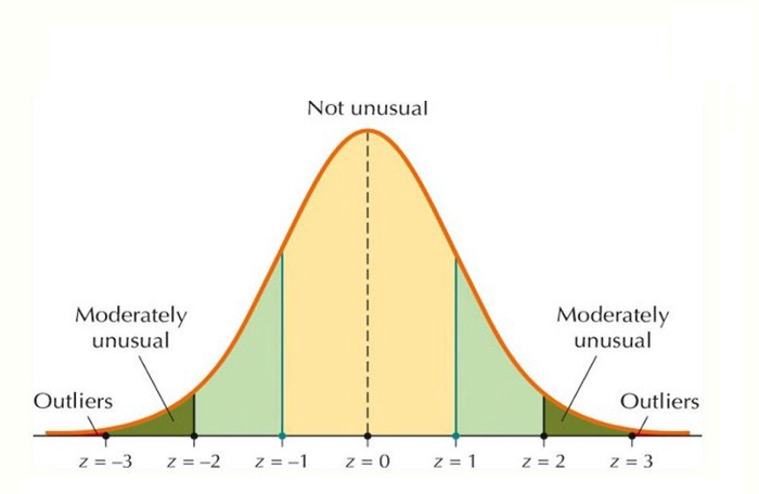
1- Z-score: the z-score, or standard score, of an observation is a metric indicating how many standard deviations a data point deviates from the mean of the sample, assuming a Gaussian distribution. This renders the z-score a parametric method. Often, data points do not conform to a Gaussian distribution, and this challenge can be addressed by applying transformations to the data, such as scaling. Python libraries like Scipy and Sci-kit Learn offer user-friendly functions and classes for easy implementation, alongside Pandas and Numpy. After appropriately transforming the selected feature space of the dataset, the z-score of any data point can be calculated using the following expression:
z = (Data Point - Mean / Sd)
When computing the z-score for each sample in the dataset, a threshold must be specified. Commonly used ‘thumb-rule’ thresholds include 2.5, 3, 3.5, or more standard deviations.
By ‘tagging’ or removing data points that fall beyond a specified threshold, we categorize the data into outliers and non-outliers. The Z-score method is a straightforward yet potent approach for handling outliers in data, particularly when dealing with parametric distributions in a low-dimensional feature space. In nonparametric scenarios, methods like DBSCAN and Isolation Forests can serve as effective solutions.
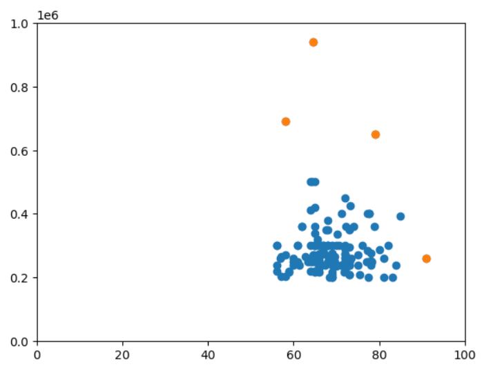
Z-score coding:
###Z-score
from scipy import stats
import pandas as pd
df = pd.read_csv('Placement_data_full_class.csv')
df=df.dropna()
df.index=[i for i in range(0,148)]#reindexing | change accordingle to reset index of df
d=pd.DataFrame(stats.zscore(df['salary']),columns=['z_score'])
d=d[(d['z_score']>3) | (d['z_score']<-3)]


degree=[]
salary=[]
for i in df.index:
    if( i in d.index):
        salary.append(df.loc[i]['salary'])
        degree.append(df.loc[i]['degree_p'])


import matplotlib.pyplot as plt
plt.scatter(df['degree_p'],df['salary'])
plt.scatter(degree,salary)
plt.show()
2- Isolation forest: The nomenclature of this technique derives from its core concept. The algorithm individually examines each data point, categorizing them into outliers or inliers based on the time it takes to isolate them. To elaborate further for clarity: when attempting to isolate a point that is evidently not an outlier, it will be surrounded by many other points, making isolation challenging. Conversely, if the point is an outlier, it stands alone, making isolation relatively straightforward. The detailed explanation of the isolation process will be provided later; your patience is appreciated.
procedure:
1- Select the point to isolate.
2- For each feature, set the range to isolate between the minimum and the maximum.
3- Choose a feature randomly.
4- Pick a value that’s in the range, again randomly
If the chosen value keeps the point above, switch the minimum of the range of the feature to the value.
If the chosen value keeps the point below, switch the maximum of the range of the feature to the value.
5- Repeat steps 3 & 4 until the point is isolated. That is, until the point is the only one which is inside the range for all features.
6- Count how many times you’ve had to repeat steps 3 & 4. We call this quantity the isolation number.
The algorithm asserts that a point is considered an outlier if it doesn’t require iteration through steps 3 and 4 multiple times.
It’s important to note that the provided pseudocode is a simplified representation of the actual process for better comprehension. In reality, since the algorithm involves the use of random numbers, this procedure is executed multiple times, and the ultimate isolation score is a composite of all the isolation scores obtained through these iterations.
Coding:
###Isolation Forest
from sklearn.ensemble import IsolationForest
df = pd.read_csv('Placement_data_full_class.csv')
df=df.dropna()
df.index=[i for i in range(0,148)]#reindexing
model=IsolationForest(n_estimators=50, max_samples='auto', contamination=float(0.05),max_features=1.0)
model.fit(df[['ssc_p']],df[['hsc_p']])
dg=pd.DataFrame({'ssc_p':df['ssc_p'],
'score':model.decision_function(df[['ssc_p']]),
'anomaly':model.predict(df[['ssc_p']]),
'hsc_p':df['hsc_p']})
import matplotlib.pyplot as plt
dg2=dg[dg['anomaly']==-1]
dg2
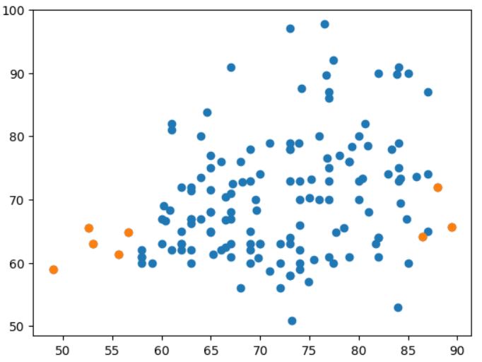
plt.scatter(dg['ssc_p'],dg['hsc_p'])
plt.scatter(dg2['ssc_p'],dg2['hsc_p'])
plt.show()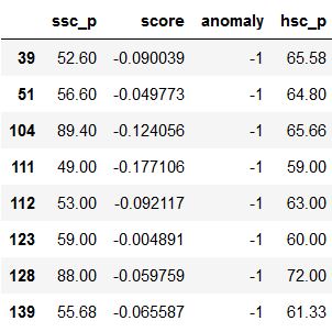
3- DBScane Anomaly Detection: As its name implies, DBSCAN (Density-Based Spatial Clustering of Applications with Noise) is a density-based and unsupervised machine learning algorithm. It processes multi-dimensional data, clustering them based on model parameters such as epsilon and minimum samples. Using these parameters, the algorithm decides whether specific values in the dataset qualify as outliers.
DBSCAN consolidates densely grouped data points into a single cluster. It excels in identifying clusters within large spatial datasets by assessing the local density of data points. Notably, DBSCAN exhibits robustness to outliers. Unlike K-Means, where the number of centroids must be predetermined, DBSCAN does not require the a priori specification of the number of clusters.
DBSCAN relies on two key parameters: epsilon and minPoints. Epsilon represents the radius of the circle formed around each data point to assess density, and minPoints denotes the minimum number of data points needed within that circle for the data point to be labeled as a Core point.
In higher dimensions, the circle transforms into a hypersphere, where epsilon becomes the radius of the hypersphere, and minPoints remains the minimum required number of data points within that hypersphere.
Here, we have a set of data points depicted in grey. Let’s observe how DBSCAN organizes and groups these data points into clusters.

DBSCAN forms a circle with an epsilon radius around each data point and categorizes them into Core points, Border points, and Noise. A data point is identified as a Core point if the circle around it encompasses at least the specified ‘minPoints’ number of points. If the count of points is below the minPoints threshold, it is labeled as a Border Point. In cases where there are no other data points within the epsilon radius of a particular data point, it is designated as Noise.

The depicted illustration illustrates a cluster generated by DBSCAN with a specified minPoints value of 3. In this context, a circle with an equal radius (epsilon) is drawn around each data point. These two parameters play a crucial role in forming spatial clusters.
Data points with a minimum of 3 points, including the point itself, within the circle are designated as Core points, distinguished by the color red. Data points with fewer than 3 but more than 1 point, including itself, within the circle are categorized as Border points, represented by the color yellow. Lastly, data points with no other points aside from itself within the circle are identified as Noise, depicted by the color purple.
Coding:
## DBScane Anomaly Detection
df = pd.read_csv('Placement_data_full_class.csv')
df=df.dropna()[['degree_p','salary']]
df.index=[i for i in range(0,148)] #reindexing | change accordingle to reset index of df


#before DBSCAN you must scale your dataset
stscaler = StandardScaler().fit(df)
df = pd.DataFrame(stscaler.transform(df))

dbsc = DBSCAN(eps = 1.3, min_samples = 25).fit(df)
labels = dbsc.labels_
outliers=df[dbsc.labels_==-1]

plt.scatter(df[0],df[1])
plt.scatter(outliers[0],outliers[1])
plt.xlabel("Degree_p")
plt.ylabel("salary")
plt.show()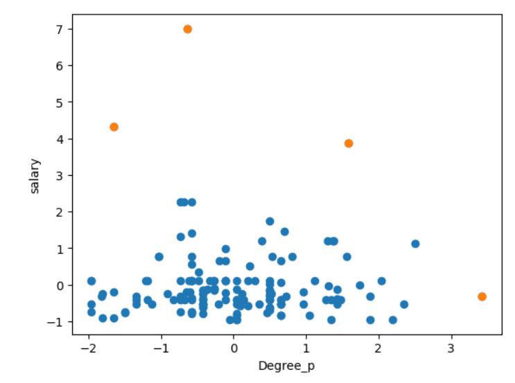
All codes:
#Step-1: Importing Necessary Dependencies

import numpy as np
import pandas as pd
import matplotlib.pyplot as plt
from sklearn.cluster import DBSCAN
import pandas as pd
from collections import Counter
from sklearn.preprocessing import StandardScaler
import numpy as np
import seaborn as sns

#Step-2: Read and Load the Dataset
df = pd.read_csv('Placement_data_full_class.csv')


plt.figure(figsize=(16,5))
plt.subplot(2,3,1)
sns.distplot(df['degree_p'])
plt.subplot(2,3,2)
sns.distplot(df['salary'])
plt.subplot(2,3,3)
sns.distplot(df['hsc_p'])
plt.subplot(2,3,4)
sns.distplot(df['ssc_p'])
plt.subplot(2,3,5)
sns.distplot(df['mba_p'])
plt.subplot(2,3,6)
sns.distplot(df['etest_p'])
plt.show()

import matplotlib.pyplot as plt
plt.scatter(df['degree_p'],df['salary'])
plt.xlim(0,100)
plt.ylim(0,1000000)
plt.show()


#Step-4: Finding the Boundary Values
Highest_allowed_degree=df['degree_p'].mean() + 3*df['degree_p'].std()
Lowest_allowed_degree=df['degree_p'].mean() - 3*df['degree_p'].std()
Highest_allowed_Salary=df['salary'].mean() + 3*df['salary'].std()
Lowest_allowed_Salary=df['salary'].mean() - 3*df['salary'].std()

print("Highest allowed_degree",Highest_allowed_degree)
print("Lowest allowed_degree : ",Lowest_allowed_degree)
print("Highest allowed Salary",Highest_allowed_Salary)
print("Lowest allowed Salary",Lowest_allowed_Salary)

#Step-5: Finding the Outliers
Outlier_data=df[(df['salary'] > Highest_allowed_Salary) | (df['salary'] < Lowest_allowed_Salary)].append(df[(df['degree_p'] > Highest_allowed_degree) | (df['degree_p'] < Lowest_allowed_degree)])


#plot outliers
import matplotlib.pyplot as plt
plt.scatter(df['degree_p'],df['salary'])
plt.scatter(Outlier_data['degree_p'],Outlier_data['salary'])
#changel lim according to your data
plt.xlim(0,100)
plt.ylim(0,1000000)
plt.show()

## Capping

df_c=df.copy()
df_c['degree_p'][df_c['degree_p']>Highest_allowed_degree]=Highest_allowed_degree
df_c['degree_p'][df_c['degree_p']<Lowest_allowed_degree]=Lowest_allowed_degree

df_c['salary'][df_c['salary']>Highest_allowed_Salary]=Highest_allowed_Salary
df_c['salary'][df_c['salary']<Lowest_allowed_Salary]=Lowest_allowed_Salary


#plot outliers
plt.scatter(df_c['degree_p'],df_c['salary'])
plt.xlim(0,100)
plt.ylim(0,1000000)
plt.show()
plt.scatter(df['degree_p'],df['salary'])
plt.scatter(Outlier_data['degree_p'],Outlier_data['salary'])
#changel lim according to your data
plt.xlim(0,100)
plt.ylim(0,1000000)
plt.show()


## Triming
#just apply pands dataframe filter
df_t=df.copy()
df_t=df_t[(df_t['salary'] < Highest_allowed_Salary) & (df_t['salary'] > Lowest_allowed_Salary)]
df_t=df_t[(df_t['degree_p'] < Highest_allowed_degree) & (df_t['degree_p'] > Lowest_allowed_degree)]
plt.scatter(df_t['degree_p'],df_t['salary'])
plt.xlim(0,100)
plt.ylim(0,1000000)
plt.show()
plt.scatter(df['degree_p'],df['salary'])
plt.scatter(Outlier_data['degree_p'],Outlier_data['salary'])
#changel lim according to your data
plt.xlim(0,100)
plt.ylim(0,1000000)
plt.show()


## Considering as missing value
df_n=df.copy()
df_n['salary'][(df_n['salary'] >= Highest_allowed_Salary) | (df_n['salary'] <= Lowest_allowed_Salary)]=np.nan
df_n['degree_p'][(df_n['degree_p'] >= Highest_allowed_degree) | (df_n['degree_p'] <= Lowest_allowed_degree)]=np.nan


###Z-score
from scipy import stats
import pandas as pd
df = pd.read_csv('Placement_data_full_class.csv')
df=df.dropna()
df.index=[i for i in range(0,148)]#reindexing | change accordingle to reset index of df
d=pd.DataFrame(stats.zscore(df['salary']),columns=['z_score'])
d=d[(d['z_score']>3) | (d['z_score']<-3)]


degree=[]
salary=[]
for i in df.index:
    if( i in d.index):
        salary.append(df.loc[i]['salary'])
        degree.append(df.loc[i]['degree_p'])


import matplotlib.pyplot as plt
plt.scatter(df['degree_p'],df['salary'])
plt.scatter(degree,salary)
plt.show()


###Isolation Forest

from sklearn.ensemble import IsolationForest
df = pd.read_csv('Placement_data_full_class.csv')
df=df.dropna()
df.index=[i for i in range(0,148)]#reindexing
model=IsolationForest(n_estimators=50, max_samples='auto', contamination=float(0.05),max_features=1.0)
model.fit(df[['ssc_p']],df[['hsc_p']])

dg=pd.DataFrame({'ssc_p':df['ssc_p'],
                 'score':model.decision_function(df[['ssc_p']]),
                 'anomaly':model.predict(df[['ssc_p']]),
                 'hsc_p':df['hsc_p']})
import matplotlib.pyplot as plt
dg2=dg[dg['anomaly']==-1]
dg2

plt.scatter(dg['ssc_p'],dg['hsc_p'])
plt.scatter(dg2['ssc_p'],dg2['hsc_p'])
plt.show()


## DBScane Anomaly Detection
df = pd.read_csv('Placement_data_full_class.csv')
df=df.dropna()[['degree_p','salary']]
df.index=[i for i in range(0,148)] #reindexing | change accordingle to reset index of df


#before DBSCAN you must scale your dataset
stscaler = StandardScaler().fit(df)
df = pd.DataFrame(stscaler.transform(df))

dbsc = DBSCAN(eps = 1.3, min_samples = 25).fit(df)
labels = dbsc.labels_
outliers=df[dbsc.labels_==-1]

plt.scatter(df[0],df[1])
plt.scatter(outliers[0],outliers[1])
plt.xlabel("Degree_p")
plt.ylabel("salary")
plt.show()


### Elliptic Envelope

from sklearn.covariance import EllipticEnvelope
import pandas as pd
df = pd.read_csv('Placement_data_full_class.csv')
df=df.dropna()[['degree_p','salary']]
df.index=[i for i in range(0,148)]#reindexing | change accordingle to reset index of df