Probability Theory (Naïve Bayes Classification)
In this blog, we will first represent an introduction to the Bayes theorem, the foundation of Bayes classifier. Then it is learnt how to create and assess a Naïve Bayes classifier using Python Sklearn module.
Bayes’ theorem is a simple mathematic formula used for calculating conditional probability. Its formula is:
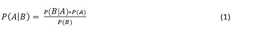
P(A|B): The probability of event A occurring given that B is true (posterior probability of A given B)
P(B|A): The probability of event A occurring given that B is true (posterior probability of A given B)
Example: watching movies based on genre
Results are based as bellow
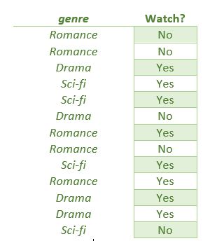
Frequency and probability table:
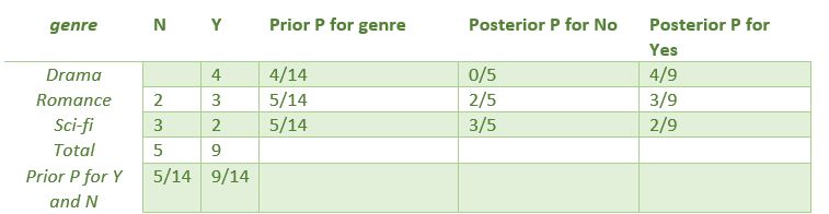
Calculating the probability of watching the genre of Drama
P(Yes|Drama) = P(Drama|Yes) * P(Yes)/P(Drama)
P(Drama) = 4/14, P(Yes) = 9/14, P(Overcast|Yes) = 4/9
So,
P(Yes|Drama) = 0.98
Similarly, not watching the Drama genre
P(No|Drama) = P(Drama|No) * P(No)/P(Drama)
P(Drama) = 4/14, P(No) = 5/14, P(Overcast|No) = 0/5
So,
P(No|Drama) = 0
The probability of ‘yes’ class is higher. So if the film is in drama genre, it will be watched
In case of having multiple characteristics to calculating probability the Bayes’ classifier obey the following steps:
Calculate prior probability for given class table
Calculate conditional probability with each feature for each class
Multiply same class conditional probability
Multiply prior probability with previous step probability
See which class has higher probability
For example if we include the price of movies on our decision to watch it or not (Price = expensive, reasonable and cheap)
P(Yes | Drama, Reasonable) = P(Drama, Reasonable | Yes) * P(Yes) ….. (For comparison with do not need the denominator)
P(No | Drama, Reasonable) = (Drama, Reasonable | No) * P(No) ….
Training and assessment of Bayes’ Classifier module on artificially manufactured data (Synthetic data)
Data Generation
Artificial data generation is often useful when there is no real-world data or real information are kept private due to compliance risks.
Sklearn module enable us to generate synthetic information using make_classification function. Synthetic data are customizable, which means it is possible to create data that meet our needs. In this case, we are begetting a dataset with a desired numbers of classes, features and samples.
## Generating the Dataset

from sklearn.datasets import make_classification

X, y = make_classification(
    n_features=6,
    n_classes=3,
    n_samples=800,
    n_informative=2,
    random_state=1,
    n_clusters_per_class=1,
)
Code explanation:
Import the make_classification function from sklearn module
Make_classification function generate a random dataset for classification projects
Function arguments: n_features: number of independent variables; n_class: the number of target variables; n_samples: the number of observations; n-Informative: the number of influential features on target variables; random_state: ensuring that dataset is reproducible; n_clusster_per_class: determine the degree of separation between the classes.
X: features of dataset
y: target variables
Visualization of dataset importing scatter functions from matplotlib module
## visualize the dataset

import matplotlib.pyplot as plt

plt.scatter(X[:, 0], X[:, 1], c=y, marker="*");
Code explanation:
import scatter from matplotlib
scatter function takes first and second columns of X array; c=y provides colors for each data point; marker assign a shaper for each of data point.
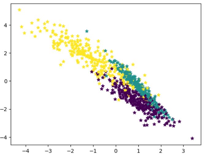
As you can see there are three target labels (Multiclass classification model)
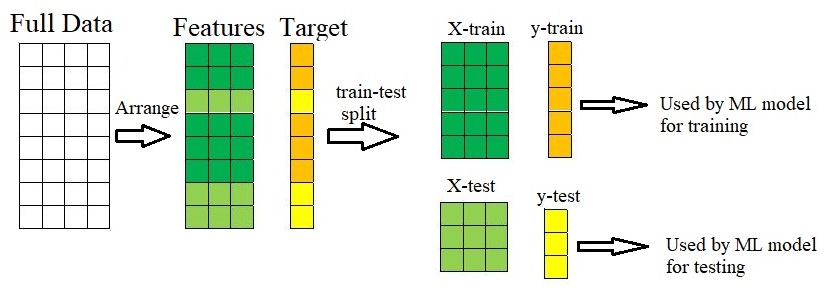
Train and test datasets
A proficient supervised model excels in delivering accurate predictions on new data. The availability of fresh data facilitates the assessment of model performance. Nevertheless, in situations where new information is unavailable, it proves beneficial to partition the existing data into two sets: training and testing.
The train-test procedure is spelled out in the bellow figure:
## Train Test Split

from sklearn.model_selection import train_test_split

X_train, X_test, y_train, y_test = train_test_split(
    X, y, test_size=0.33, random_state=125
)
Code explanation:
import train_test_split function from sklearn module
train_test_split function arguments: X (input features), y (target variables), test_size (proportion of test size) and random_size
In the next step, we build the Gaussian Naïve Bayes model, train it and make prediction:
from sklearn.naive_bayes import GaussianNB

# Build a Gaussian Classifier
model = GaussianNB()

# Model training
model.fit(X_train, y_train)
Both actual and predicted values and the same:
# Predict Output
predicted = model.predict([X_test[6]])

print("Actual Value:", y_test[6])
print("Predicted Value:", predicted[0])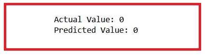
Model assessment
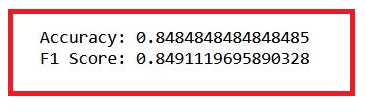
We make a prediction of test dataset and then calculate the accuracy and F1-score (a criteria for precision and recall):
Importing several functions from the sklearn.metrics module, including accuracy_score, confusion_matrix, ConfusionMatrixDisplay, and f1_score
Making prediction is done by model.predict
Based on values for accuracy and f1-score, we concluded our model works properly.
True positive and true negative are calculated by confusion_matrix and visualized by ConfusionMatrixDisplay.
Our model performed in a good way. However, there are some ways to improve it more like scaling, cross-validation and hyperparameter optimization.
## Model Evaluation

from sklearn.metrics import (
    accuracy_score,
    confusion_matrix,
    ConfusionMatrixDisplay,
    f1_score,
)

y_pred = model.predict(X_test)
accuray = accuracy_score(y_pred, y_test)
f1 = f1_score(y_pred, y_test, average="weighted")

print("Accuracy:", accuray)
print("F1 Score:", f1)

## visualize the Confusion matrix

labels = [0,1,2]
cm = confusion_matrix(y_test, y_pred, labels=labels)
disp = ConfusionMatrixDisplay(confusion_matrix=cm, display_labels=labels)
disp.plot();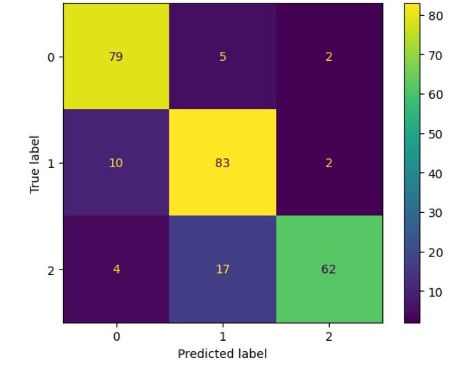
All codes:
## Generating the Dataset

from sklearn.datasets import make_classification

X, y = make_classification(
    n_features=6,
    n_classes=3,
    n_samples=800,
    n_informative=2,
    random_state=1,
    n_clusters_per_class=1,
)

## visualize the dataset

import matplotlib.pyplot as plt

plt.scatter(X[:, 0], X[:, 1], c=y, marker="*");

## Train Test Split

from sklearn.model_selection import train_test_split

X_train, X_test, y_train, y_test = train_test_split(
    X, y, test_size=0.33, random_state=125
)

from sklearn.naive_bayes import GaussianNB

# Build a Gaussian Classifier
model = GaussianNB()

# Model training
model.fit(X_train, y_train)

# Predict Output
predicted = model.predict([X_test[6]])

print("Actual Value:", y_test[6])
print("Predicted Value:", predicted[0])

## Model Evaluation

from sklearn.metrics import (
    accuracy_score,
    confusion_matrix,
    ConfusionMatrixDisplay,
    f1_score,
)

y_pred = model.predict(X_test)
accuray = accuracy_score(y_pred, y_test)
f1 = f1_score(y_pred, y_test, average="weighted")

print("Accuracy:", accuray)
print("F1 Score:", f1)

## visualize the Confusion matrix

labels = [0,1,2]
cm = confusion_matrix(y_test, y_pred, labels=labels)
disp = ConfusionMatrixDisplay(confusion_matrix=cm, display_labels=labels)
disp.plot();