Regression Machine Learning Methods

In this post, we use some regression machine learning methods on a dataset and make a comparison of outcomes for different methods.  The applying methods are 1- Random Forest Regression 2- Support Vector Regression (SVR) 3- Multiple Linear Regression and 4- Linear Regression

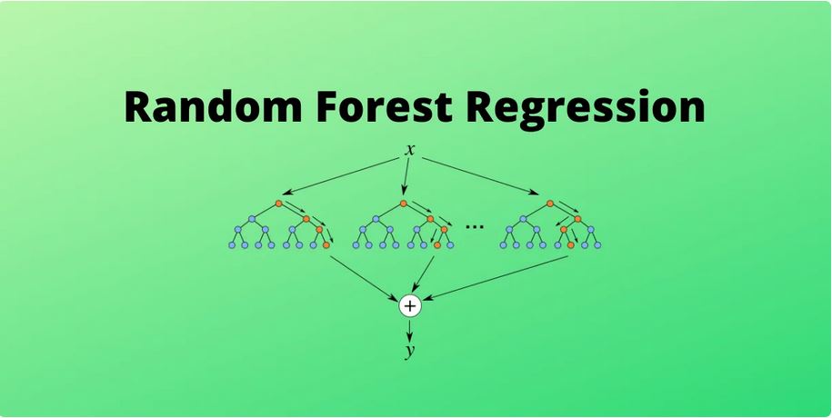
1- Random Forest Regression is a supervised learning algorithm and bagging technique within machine learning that utilizes an ensemble learning method for regression. The trees in Random Forests run in parallel, implying no interaction between these trees during their construction.

Random Forest Regression is a supervised learning algorithm employing an ensemble learning approach for regression.

It’s important to note that Random Forest is a bagging technique rather than a boosting technique. The trees in Random Forests operate in parallel, indicating that there is no interaction between these trees during the tree-building process.

2- Support Vector Regression (SVR): Support Vector Regression (SVR) represents a machine learning algorithm employed in regression analysis. Its objective is to identify a function that estimates the connection between input variables and a continuous target variable, with a focus on minimizing prediction errors.

In contrast to Support Vector Machines (SVMs) utilized for classification purposes, SVR aims to locate a hyperplane that optimally accommodates data points in a continuous space. This involves mapping input variables to a high-dimensional feature space and determining the hyperplane that maximizes the margin (distance) from the hyperplane to the nearest data points, all while minimizing prediction errors.

SVR exhibits the capability to address non-linear associations between input variables and the target variable through the incorporation of a kernel function, facilitating the mapping of data to a higher-dimensional space. This characteristic renders SVR particularly potent for regression tasks characterized by intricate relationships between input variables and the target variable.

Hyperparameters of the Support Vector Regression (SVR) and Support Vector Machine (SVM) Algorithms:

• Kernel: Utilizing a kernel aids in identifying a hyperplane within a higher-dimensional space without escalating the computational cost. Typically, the computational cost rises as the dimension of the data increases. This escalation in dimensionality becomes necessary when a separating hyperplane cannot be found within the given dimension, compelling the need to transition to a higher-dimensional space.

• Hyperplane:In SVM, this essentially represents a demarcating line between two classes of data. However, in Support Vector Regression, this line serves as the basis for predicting continuous output values.

• Decision Boundary: A decision boundary can be conceptualized as a demarcation line (for simplicity), with positive examples on one side and negative examples on the other. Along this line, examples may be classified as either positive or negative. This identical concept from SVM is also employed in Support Vector Regression.

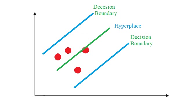
There are many hyperplanes to separate the data, but in SVR, we look for a hyperplane with the maximum margin (distance) between two classes. So we choose the hyperplane so that the distance from it to the nearest data point on each side is maximized. (for support vector machine)

Envision the two blue lines as the decision boundary, with the green line serving as the hyperplane. In the context of SVR, our aim is primarily focused on the points situated within the decision boundary line. The optimal fit line corresponds to the hyperplane that encompasses the maximum number of points.

3&4- Multiple Linear Regression and Linear Regression: Linear regression referred to as simple regression, linear regression establishes a connection between two variables. Graphically, linear regression is represented by a straight line, where the slope defines how changes in one variable influence changes in the other. The y-intercept in a linear regression relationship signifies the value of one variable when the other variable is 0. In instances of intricate connections within data, the relationship may be elucidated by more than a single variable. In such cases, analysts employ multiple regression, a technique aimed at elucidating a dependent variable by considering multiple independent variables.

After getting familiarized with different machine learning regression model, we will start to use those models on real life data.

Importing our needed libraries:

## Importing the libraries
import pandas as pd
import numpy as np
import seaborn as sns
import matplotlib.pyplot as plt
from sklearn.impute import SimpleImputer
from sklearn.metrics import r2_score
from sklearn.preprocessing import StandardScaler
from sklearn.model_selection import train_test_split
from sklearn.ensemble import RandomForestRegressor
from sklearn.preprocessing import PolynomialFeatures
from sklearn.linear_model import LinearRegression
from sklearn.tree import DecisionTreeRegressor
from sklearn.svm import SVR

Fixing column names:

## Importing the dataset

data = pd.read_csv("Life Expectancy Data.csv")


## Correcting column names

column = data.columns.to_list()


data.columns = [a.strip() for a in column]

Strip (): Remove spaces at the beginning and at the end of the string

Handling missing data:

## Taking care of missing data
imputer = SimpleImputer(missing_values=np.nan, strategy="median")
data['Life expectancy'] = imputer.fit_transform(data[['Life expectancy']])
data['Adult Mortality'] = imputer.fit_transform(data[['Adult Mortality']])
data['Alcohol'] = imputer.fit_transform(data[['Alcohol']])
data['Hepatitis B'] = imputer.fit_transform(data[['Hepatitis B']])
data['BMI'] = imputer.fit_transform(data[['BMI']])
data['Polio'] = imputer.fit_transform(data[['Polio']])
data['Total expenditure'] = imputer.fit_transform(data[['Total expenditure']])
data['Diphtheria'] = imputer.fit_transform(data[['Diphtheria']])
data['GDP'] = imputer.fit_transform(data[['GDP']])
data['Population'] = imputer.fit_transform(data[['Population']])
data['thinness  1-19 years'] = imputer.fit_transform(data[['thinness  1-19 years']])
data['thinness 5-9 years'] = imputer.fit_transform(data[['thinness 5-9 years']])
data['Income composition of resources'] = imputer.fit_transform(data[['Income composition of resources']])
data['Schooling'] = imputer.fit_transform(data[['Schooling']])

Sklearn_impute_SimpleImputer: Utilizing a univariate imputer to fill in missing values through straightforward strategies. This involves replacing missing values within each column using a descriptive statistic like mean, median, or the most frequent value, or alternatively, using a constant value.

Encoding of dependent variables:

## Encoding of dependent variables
country_dummy = pd.get_dummies(data['Country'], drop_first = True)
status_dummy = pd.get_dummies(data['Status'], drop_first = True)

data.drop(['Country', 'Status'], inplace = True, axis = 1)

corr_data = data.copy()

get_dummies: Convert categorical variable into dummy/indicator variables.  Each variable is converted in as many 0/1 variables as there are different values. Columns in the output are each named after a value; if the input is a DataFrame, the name of the original variable is prepended to the value

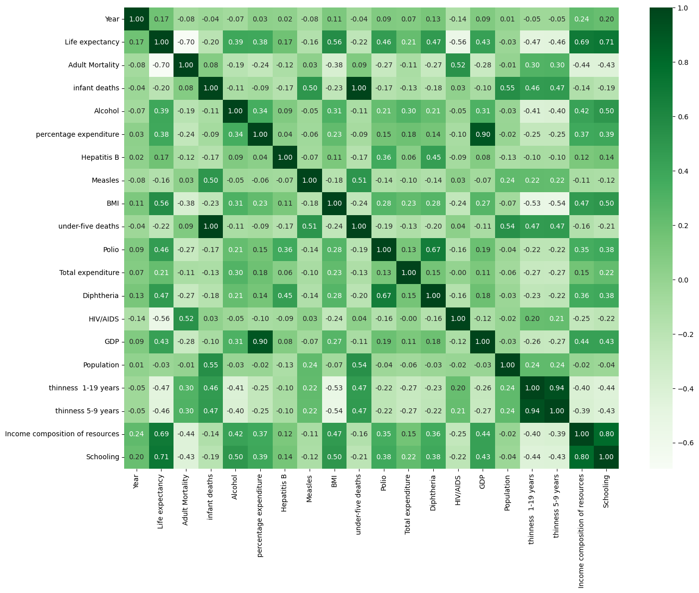
A correlation matrix is a statistical tool employed to assess the relationship between two variables within a dataset. Represented as a table, each cell in the matrix contains a correlation coefficient. A coefficient of 1 signifies a strong positive relationship between variables, 0 indicates a neutral relationship, and -1 suggests a strong negative relationship.

## Correlation matrix
correlation_matrix = corr_data.corr()

plt.figure(figsize=(16,12))
sns.heatmap(correlation_matrix, annot=True,fmt=".2f", cmap="Greens")
plt.show()

Here we have the correlation matrix for our data:

Split arrays or matrices into random train and test subsets with test size of 20%:

## Splitting the dataset into the Training set and Test set
Y = pd.DataFrame(data['Life expectancy'], columns = ['Life expectancy'])
data.drop(['Life expectancy'], inplace = True, axis = 1)

all_data = pd.concat([data, country_dummy, status_dummy], axis = 1)

X_train, X_test, y_train, y_test = train_test_split(all_data, Y, test_size = 0.2, random_state = 0)

y_test.columns = ['y_test']

Implement, prediction and evaluation of Random Forest Regression:

## Random Forest Regression model
regressor = RandomForestRegressor(n_estimators = 10, random_state = 0)
regressor.fit(X_train, y_train.values.ravel())

#Predicting the Test set results
y_pred = pd.DataFrame(regressor.predict(X_test), columns= ['y_pred'])

y_test.index = y_pred.index

random_forest_result = pd.concat([y_pred, y_test], axis = 1)


# Evaluating the Model Performance
r2_random_forest = r2_score(y_test, y_pred)

Implement, prediction and evaluation of Support Vector Regression (SVR):

##Support Vector Regression (SVR) model
# Feature scaling
sc_X = StandardScaler()
sc_y = StandardScaler()
X_train_scaled = sc_X.fit_transform(X_train)
y_train_scaled = sc_y.fit_transform(y_train)

regressor = SVR(kernel = 'rbf')
regressor.fit(X_train_scaled, y_train_scaled.ravel())

##Predicting the Test set results
y_pred = regressor.predict(sc_X.transform(X_test))
y_pred = pd.DataFrame(sc_y.inverse_transform(pd.DataFrame(y_pred)), columns= ['y_pred'])

y_test.index = y_pred.index

svr_result = pd.concat([y_pred, y_test], axis = 1)

# Evaluating the Model Performance

r2_svm = r2_score(y_test, y_pred)

Implement, prediction and evaluation of Multiple Linear Regression:

##Multiple Linear Regression model
regressor = LinearRegression()
regressor.fit(X_train, y_train)

# Predicting the Test set results

y_pred = pd.DataFrame(regressor.predict(X_test), columns= ['y_pred'])

y_test.index = y_pred.index

random_forest_result = pd.concat([y_pred, y_test], axis = 1)

# Evaluating the Model Performance

r2_multiple_linear_regression = r2_score(y_test, y_pred)

Implement, prediction and evaluation of Decision Tree Regression:

## Decision Tree Regression model
regressor = DecisionTreeRegressor(random_state = 0)
regressor.fit(X_train, y_train)

# Predicting the Test set results

y_pred = pd.DataFrame(regressor.predict(X_test), columns= ['y_pred'])

y_test.index = y_pred.index

random_forest_result = pd.concat([y_pred, y_test], axis = 1)

# Evaluating the Model Performance

r2_decision_tree_regression = r2_score(y_test, y_pred)

Implement, prediction and evaluation of Linear Regression:

def flatten(l):
    return [item for sublist in l for item in sublist]
# Set up and fit the linear regressor
lin_reg = LinearRegression()
lin_reg.fit(X_train, y_train)

# Flatten the prediction and expected lists
predicted = flatten(lin_reg.predict(X_test))
expected = flatten(y_test.values)

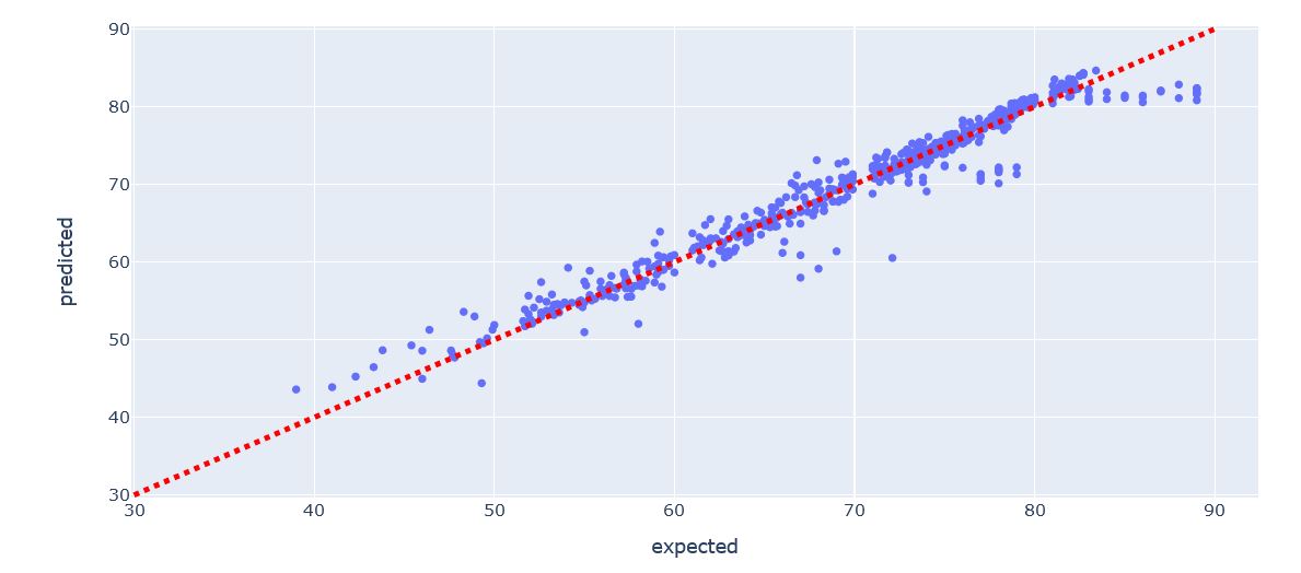
import plotly.express as px

# Put data to plot in dataframe
df_plot = pd.DataFrame({'expected':expected, 'predicted':predicted})

# Make scatter plot from data
fig = px.scatter(
    df_plot, 
    x='expected', 
    y='predicted',
    title='Predicted vs. Actual Values')

# Add straight line indicating perfect model
fig.add_shape(type="line",
    x0=30, y0=30, x1=90, y1=90,
    line=dict(
        color="Red",
        width=4,
        dash="dot",
    )
)

# Show figure
fig.show()
error = np.sqrt(np.mean((np.array(predicted) - np.array(expected)) ** 2))
print(f"RMS: {error:.4f} ")

r2=r2_score(expected, predicted)
print(f"R2: {round(r2,4)}") 

Comparison of model results:

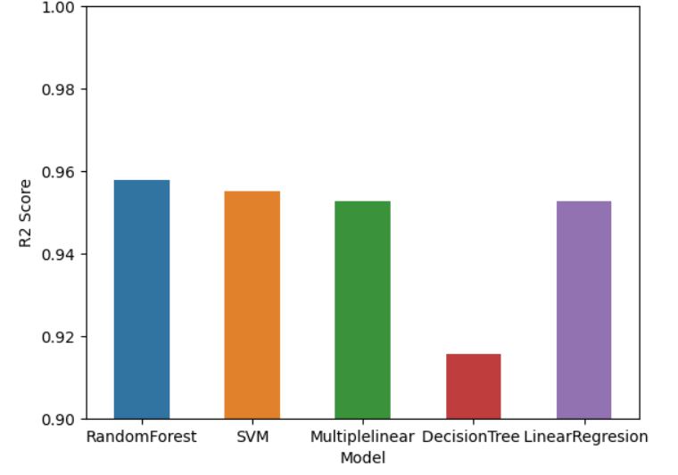
##Comparison of model results
results = pd.DataFrame([[
    r2_random_forest,
    r2_svm, 
    r2_multiple_linear_regression,
    r2_decision_tree_regression,
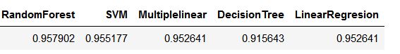
r2]], columns = ['RandomForest', 'SVM', 'Multiplelinear', 'DecisionTree ', ' LinearRegresion'])

ax = sns.barplot(results, width = 0.5)
ax.set(xlabel='Model', ylabel='R2 Score')
plt.ylim(0.9, 1)

As you can see, our models have a good prediction (R_square close to 1)

All codes:

## Importing the libraries
import pandas as pd
import numpy as np
import seaborn as sns
import matplotlib.pyplot as plt
from sklearn.impute import SimpleImputer
from sklearn.metrics import r2_score
from sklearn.preprocessing import StandardScaler
from sklearn.model_selection import train_test_split
from sklearn.ensemble import RandomForestRegressor
from sklearn.preprocessing import PolynomialFeatures
from sklearn.linear_model import LinearRegression
from sklearn.tree import DecisionTreeRegressor
from sklearn.svm import SVR

## Importing the dataset

data = pd.read_csv("Life Expectancy Data.csv")


## Correcting column names

column = data.columns.to_list()


data.columns = [a.strip() for a in column]

## Taking care of missing data
imputer = SimpleImputer(missing_values=np.nan, strategy="median")
data['Life expectancy'] = imputer.fit_transform(data[['Life expectancy']])
data['Adult Mortality'] = imputer.fit_transform(data[['Adult Mortality']])
data['Alcohol'] = imputer.fit_transform(data[['Alcohol']])
data['Hepatitis B'] = imputer.fit_transform(data[['Hepatitis B']])
data['BMI'] = imputer.fit_transform(data[['BMI']])
data['Polio'] = imputer.fit_transform(data[['Polio']])
data['Total expenditure'] = imputer.fit_transform(data[['Total expenditure']])
data['Diphtheria'] = imputer.fit_transform(data[['Diphtheria']])
data['GDP'] = imputer.fit_transform(data[['GDP']])
data['Population'] = imputer.fit_transform(data[['Population']])
data['thinness  1-19 years'] = imputer.fit_transform(data[['thinness  1-19 years']])
data['thinness 5-9 years'] = imputer.fit_transform(data[['thinness 5-9 years']])
data['Income composition of resources'] = imputer.fit_transform(data[['Income composition of resources']])
data['Schooling'] = imputer.fit_transform(data[['Schooling']])

## Encoding of dependent variables
country_dummy = pd.get_dummies(data['Country'], drop_first = True)
status_dummy = pd.get_dummies(data['Status'], drop_first = True)

data.drop(['Country', 'Status'], inplace = True, axis = 1)

corr_data = data.copy()

## Correlation matrix
##correlation_matrix = corr_data.corr()

##plt.figure(figsize=(16,12))
##sns.heatmap(correlation_matrix, annot=True,fmt=".2f", cmap="Greens")
##plt.show()

## Splitting the dataset into the Training set and Test set
Y = pd.DataFrame(data['Life expectancy'], columns = ['Life expectancy'])
data.drop(['Life expectancy'], inplace = True, axis = 1)

all_data = pd.concat([data, country_dummy, status_dummy], axis = 1)

X_train, X_test, y_train, y_test = train_test_split(all_data, Y, test_size = 0.2, random_state = 0)

y_test.columns = ['y_test']

## Random Forest Regression model
regressor = RandomForestRegressor(n_estimators = 10, random_state = 0)
regressor.fit(X_train, y_train.values.ravel())

#Predicting the Test set results
y_pred = pd.DataFrame(regressor.predict(X_test), columns= ['y_pred'])

y_test.index = y_pred.index

random_forest_result = pd.concat([y_pred, y_test], axis = 1)


# Evaluating the Model Performance
r2_random_forest = r2_score(y_test, y_pred)


##Support Vector Regression (SVR) model
# Feature scaling
sc_X = StandardScaler()
sc_y = StandardScaler()
X_train_scaled = sc_X.fit_transform(X_train)
y_train_scaled = sc_y.fit_transform(y_train)

regressor = SVR(kernel = 'rbf')
regressor.fit(X_train_scaled, y_train_scaled.ravel())

##Predicting the Test set results
y_pred = regressor.predict(sc_X.transform(X_test))
y_pred = pd.DataFrame(sc_y.inverse_transform(pd.DataFrame(y_pred)), columns= ['y_pred'])

y_test.index = y_pred.index

svr_result = pd.concat([y_pred, y_test], axis = 1)

# Evaluating the Model Performance

r2_svm = r2_score(y_test, y_pred)

##Multiple Linear Regression model
regressor = LinearRegression()
regressor.fit(X_train, y_train)

# Predicting the Test set results

y_pred = pd.DataFrame(regressor.predict(X_test), columns= ['y_pred'])

y_test.index = y_pred.index

random_forest_result = pd.concat([y_pred, y_test], axis = 1)

# Evaluating the Model Performance

r2_multiple_linear_regression = r2_score(y_test, y_pred)

## Decision Tree Regression model
regressor = DecisionTreeRegressor(random_state = 0)
regressor.fit(X_train, y_train)

# Predicting the Test set results

y_pred = pd.DataFrame(regressor.predict(X_test), columns= ['y_pred'])

y_test.index = y_pred.index

random_forest_result = pd.concat([y_pred, y_test], axis = 1)

# Evaluating the Model Performance

r2_decision_tree_regression = r2_score(y_test, y_pred)

##Comparison of model results
results = pd.DataFrame([[
    r2_random_forest,
    r2_svm, 
    r2_multiple_linear_regression,
    r2_decision_tree_regression,
r2]], columns = ['RandomForest', 'SVM', 'Multiplelinear', 'DecisionTree ', ' LinearRegresion'])

ax = sns.barplot(results, width = 0.5)
ax.set(xlabel='Model', ylabel='R2 Score')
plt.ylim(0.9, 1)





## me
def flatten(l):
    return [item for sublist in l for item in sublist]
# Set up and fit the linear regressor
lin_reg = LinearRegression()
lin_reg.fit(X_train, y_train)

# Flatten the prediction and expected lists
predicted = flatten(lin_reg.predict(X_test))
expected = flatten(y_test.values)

import plotly.express as px

# Put data to plot in dataframe
df_plot = pd.DataFrame({'expected':expected, 'predicted':predicted})

# Make scatter plot from data
fig = px.scatter(
    df_plot, 
    x='expected', 
    y='predicted',
    title='Predicted vs. Actual Values')

# Add straight line indicating perfect model
fig.add_shape(type="line",
    x0=30, y0=30, x1=90, y1=90,
    line=dict(
        color="Red",
        width=4,
        dash="dot",
    )
)

# Show figure
fig.show()
error = np.sqrt(np.mean((np.array(predicted) - np.array(expected)) ** 2))
print(f"RMS: {error:.4f} ")

r2=r2_score(expected, predicted)
print(f"R2: {round(r2,4)}")